A demonstration video on the Solvency II metrics for long tail liabilities, as discussed in the following article, is viewable here.
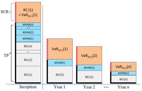
For the one-year risk horizon, risk capital is raised at the beginning of each year. The cost of raising the risk capital, the Market Value Margin (MVM) or premium on the risk capital, is paid to the capital providers at the end of each year along with any unused risk capital. The sum of the MVMs and the Best Estimate of Liabilities (BELs) for each calendar year is the Technical Provision (also referred to as Fair Value of Liabilities).
In the examples below, we assume that all capital, including the risk capital fund, is invested by the company. In the event that this is not the case, then the discount formulae for MVM are appropriately adjusted.
Risk Capital (RC) is not part of the Technical Provision (TP). Furthermore, if our Best Estimate of Liabilities (BEL) is based on suitable assumptions, then we expect that in the long term draws on the risk fund will balance out to zero; the risk capital fund operates as a form of insurance. A poor estimate of BEL, could itself result in a 'distress' year being encountered.
TP = BEL + MVM
As prescribed by the Cost of Capital method, the MVM(k) for a given future period k is the present value (PV) of the Risk Capital requirement for that period multiplied by the spread. Assuming the spread above the risk free rate is s, and the risk free rate is d, the MVM for year k is given by:
MVM(k) = s(k)*RC(k)*PV(k),
BEL(k) = E[Lk]*PV(k-0.5),
where PV(k) = 1/(1+d)k , Lk are the paid losses in year k,
and we allow that the spread may not be constant, and RC(k) is the risk capital raised at the beginning of year k, based on the model as estimated at the valuation date.
The BEL is the PV adjusted sum of the means (E[Lk]) of the calendar year liability distributions. Note that losses are paid uniformly throughout the year, so we discount for half a year.
At the end of each year k the capital providers receive
MVM(k)/PV(k),
and the risk-free interest earned on the risk capital. In addition, any unused portion of the risk fund is returned. Since MVM is held for the whole year, a full year discount is applied.
Thus, for each individual future year we have,
TP(k) = BEL(k) + MVM(k)
In aggregate:
TP = Sum(TP(k); k= 1,2...n)
The Solvency Capital Requirement (SCR) at inception includes the amount of money needed to rebalance the balance sheet after the first year in distress.
Example: Uncorrelated future calendar years
In the event that the calendar years are uncorrelated, the first year in distress does not impact the distributions of the paid losses liability streams for subsequent years.
Correlation between future calendar years
In the initial formulation, the Risk Capital for each calendar year is set equal to the Value at Risk at the 99.5-percentile (VaR<sub99.5%< sub="">), that is, the amount by which the 99.5th percentile exceeds the mean of the distribution of losses for that calendar year. This is naive as this fomulation ignores (or treats as zero) the correlations between the calendar year paid loss distributions.
Future calendar year liability stream distributions are correlated due to parameter uncertainty.
If the paid loss outcome for the first year is known to fall in to the 99.5th percentile then the (conditional) distributions for all subsequent years will be altered. The unconditional distributions must be replaced by the conditional distributions, where the condition in question is that the first year is at the 99.5th percentile. Accordingly, the technical provisions and the risk capital raised at the beginning of each year will change.
Considering only the second year, the technical provision based on the conditional distribution will be higher than the technical provision based on the unconditional distribution.
For brevity let us call this difference
ΔTP(2).
As we require the risk capital to be sufficient to not only cover the additional payments for the distressed year (VaR<sub99.5%< sub="">) but also to restore the balance sheet at the beginning of the second year, then the fund will need to be supplemented by ΔTP(2). This money is drawn from the Risk Fund at the end of year one in the event of a distress year to compensate for the change in the paid loss distribution in year two.
Similarly for all future years.
Example: Two year run-off (Correlated)
If the first year is in distress (ξ), then the conditional distributions for subsequent years change resulting in (typically) higher technical provisions.
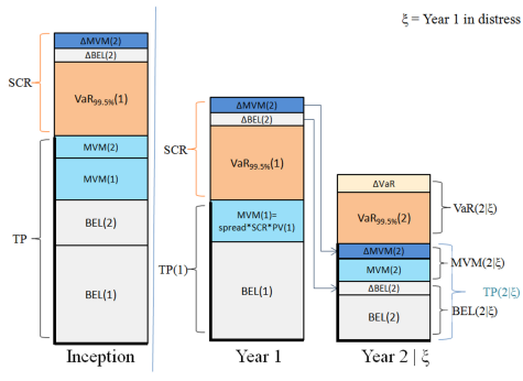
After the distress scenario for the first year (denoted ξ), our view of the mean and volatility of the loss distribution for year two has changed. The new VaR is now VaR(2|ξ)
The risk capital requirement for year two has been revised by an amount equal to
VaR(2|ξ) - VaR(2).
The cost of holding this extra risk capital we call ΔMVM(2). Similarly, the BEL for year 2 has been revised, and
ΔBEL(2) = (E[L2|ξ] - E[L2]) * PV(0.5)
is the extra amount required.
The sum of these amounts (ΔBEL(2) and ΔMVM(2)), which we call ΔTP(2), is what is needed in addition to our previously assigned provisions, TP(2), at the outset of year two in order to restore the balance sheet to health at the beginning of the second year.
This forms part of the SCR in year 1.
Note the Δ estimates are separate from our estimates of BEL(2) and MVM(2) since these adjustments to BEL(2) and MVM(2) are only incorporated if the first year is in distress; there is no recursion.
SCR = VaR99.5%(1) + ΔTP(2)
This changes MVM(1) and hence TP(1).
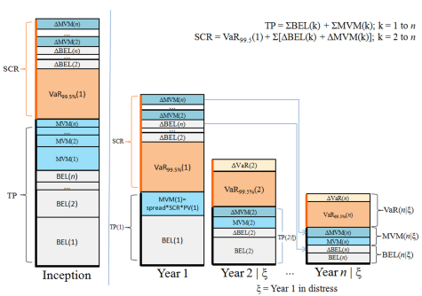
Example: n-year run-off (Correlated)
The general case is simply an extension of the two-year example.
We now adjust by ΔTP = ΔTP(2) + ΔTP(3) +...ΔTP(n),
where n is the limit of run-off.
SCR = VaR99.5%(1) + ΔTP
This changes MVM(1) and hence TP(1), however for k > 1, MVM(k) and BEL(k) are unchanged since in the event of the distress scenario, we can draw on the risk fund for the amounts ΔMVM(k) and ΔBEL(k), to augment the MVM(k) and BEL(k) appropriately.
The additional capital required to adjust the BEL is ΔBEL(k); namely
(E[Lk|ξ] - E[Lk]) * PV(0.5).
Similarly, it is anticipated that the new risk capital that needs to be raised at the beginning of year k is VaR99.5%(k|ξ).
The cost of raising this extra risk capital in year k is ΔMVM(k), based on VaR(k|ξ) - VaR(k).
If the first year is in distress...
In summary, if the first year is in distress, then the following events occur.
BEL(1) and VaR99.5%(1) are exhausted (the losses incurred were at the 99.5% quantile). No risk capital is returned to the capital providers.
MVM(1) / PV(1) (plus the risk free rate on the SCR) is returned to the capital providers. Total amount returned is: SCR*(d+s).
BEL(2) is adjusted by ΔBEL(2) at the beginning of year two; that is, E[L2|ξ] * PV(0.5) is available at the beginning of year two.
MVM(2) is adjusted by ΔMVM(2) at the beginning of year two;
MVM(2) / PV(1) + ΔMVM(2) / PV(1) is available at the beginning of year two.
We emphasise that any return on ΔBEL(k) and ΔMVM(k) in the first year is returned to the capital providers as part of the risk free rate calculated on the SCR.
Similarly, BEL(k) is adjusted by ΔBEL(k) at the beginning of year two and MVM(k) is adjusted by ΔMVM(k) at the beginning of year two for all future years (k>2).
The economic balance sheet has been restored to a fair value of liabilities at the beginning of the second year if the first year was in distress.
Consistency of Solvency II risk measures and prior year ultimates on updating
The Solvency Capital raised each year on updating, should not be subject to major shocks due to model errors.
Solvency II risk measures and estimates of prior year ultimates are statistically consistent on updating from year to year if the revised forecast assumptions are statistically equivalent with the prior assumptions. This is illustrated, in detail, here.
All the information you need to calculate Solvency II risk measures for your entire long-tail liability enterprise
Our Solvency II brochure is available here.
Fungibility of Lines of Business and Calendar Years
By default, we assume that the there is no fungibility between calendar years, but LOBs are fungible. That is, a surplus in one LOB can supplement a deficit in another LOB. In practice, this is not necessarily the case for legal or other reasons. Thus, we provide additional options to describe fungibility as follows:
- All lines are fungible, calendar years going forward are fungible (default in ICRFS-Plus™)
- Lines of business are not fungible, calendar years going forward are fungible
- All lines are fungible, calendar years are not fungible
- No fungibility either by Line of Business or by calendar year
The above options are important as they describe the level of diversification afforded for writing multiple Lines of Business - for MVM and Risk Capital. Fungibility applies to the risk capital fund and whether surpluses supplement the risk capital fund (which lowers the required risk capital) or whether the risk fund has to stand on its own.
Proportionality principle and Standard Formula
Quantitative Impact Studies QIS4 and QIS5 run by CEIOPS postulate the principle of proportionality in the Standard Formula (see for example paragraph SCR.1.3 of Technical specifications for QIS5). This principle assumes VaR is proportional to the BEL for the future years. According to the QIS5, the insurer should assess whether the proportionality principle is applicable.
Based on the research conducted in Insureware, proportionality does not hold for long-tail non-life insurance risk, manifesting the need for the Solvency II Internal model.
Using one year risk horizon metrics module in ICRFS-Plus™, the assertion of inapplicability of the proportionality principle can easily be verified.
ICRFS™ one year risk horizon metrics module
The one year risk horizon metrics module starts with the identified MPTF composite model with the associated forecasting scenario. This Solvency II brochure contains a detailed description of the calculations of the one-year risk horizon in the Solvency II context.
Demonstration videos
To view a demonstration video on Capital Management of all long tail liabilities click here.
To view a demonstration video on Solvency II metrics for long tail liabilities click here.