Thomas Mack identified the stochastic regression model that underlies volume weighted average link ratios. Other authors, including Murphy and Venter, have developed these ideas further. A graphical representation and regression formulation of link ratios makes it clear what assumptions underpin the methods and extensions thereof.
"There is pleasure in recognizing old things from a new viewpoint." - Richard Feynman
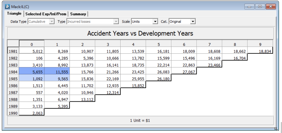
Consider the (diagonally opposite)Incurred Loss triangular data from the American Reinsurance Association.
In general, each link ratio (y/x) is the slope of the line from the number pair (x,y) to the origin.
The graph below plots the cumulatives in development year one versus the cumulatives in development year zero for accident years 1981 to 1989.
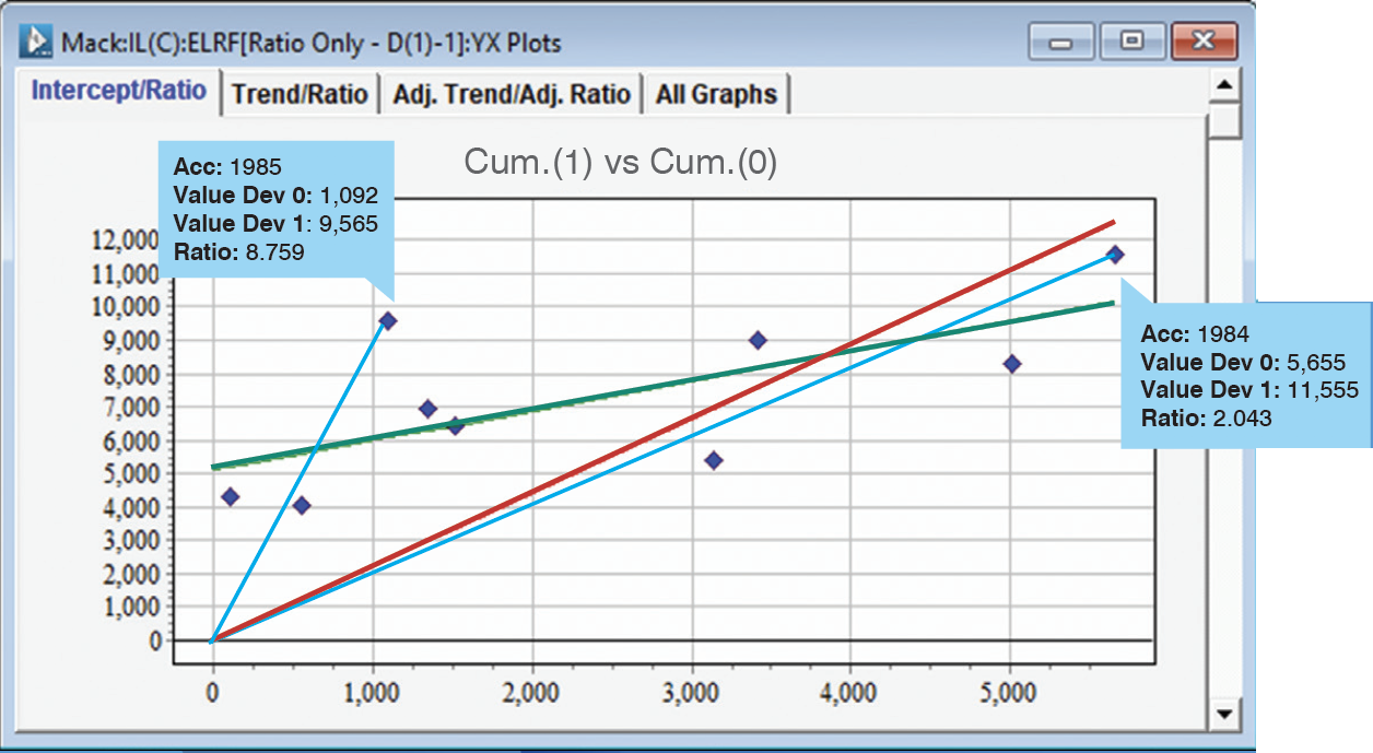
The caption on the right is for the point (5,655, 11,555) corresponding to accident year 1984. The caption on the left is for the point (1,092, 9,565) corresponding to accident year 1985. The slope of the blue lines represent the corresponding link ratios – which is 2.043 for 1984 and 8.759 for 1985.
Accordingly, an average link ratio, equivalently average trend, is an average slope through the origin.
This means that the method can be formulated as a regression (Mack (1993)).
Let y(w) denote the cumulative in development period j for accident year w and x(w) the cumulative in the previous development period, j-1.
We can write,
y(w) = b * x(w) + e(w),… (1)
where b is the slope of the line (equivalently, the average link ratio), and e(w) is the difference between the actual value y(w) and the corresponding point on the average link ratio line (b * x(w)).
When actuaries use link ratios there are two critical assumptions:
- The expected value of the next cumulative is conditional on the previous cumulative multiplied by an unknown factor.
- The selected link ratio (factor) is optimal for prediction.
The optimum value of b is found by weighted least squares estimation according to the scale of the error terms e(w).
Let the variance of e(w) = v * x(w)^delta
For the following values of delta (0, 1, 2):
- 0, or constant variance, the weighted least squares estimated of b is the volume squared weighted average link ratio.
- 1, the weighted least squares estimate of b is the volume weighted average link ratio – sometimes called the chain ladder ratio.
- 2, the weighted least squares estimate of b is the arithmetic average link ratio.
In the graph (previous page), the red line is the best least squares line through the origin and the green line is the best least squares line that includes an intercept. The latter appears to be a better model.
Murphy (1994) extended the regression formulation to include an intercept term.
y(w) = a + b * x(w) + e(w), … (2)
where a is the intercept term, but b is no longer the average link ratio.
Given that the intercept is positive in the previous graph, the slope of the line with an intercept term is less than any average link ratio (through the origin).
We can obtain visual indications of whether a line with an intercept (Murphy (1994) method) or a line through the origin (Mack (1993) method) is better.
Most importantly, the focus should be on the incremental model, Venter(1998), even if a = 0:
y(w) – x(w) = a + (b-1)*x(w) + e(w), … (3)
where y(w) – x(w) is the incremental data point.
When you use a link ratio to project the cumulative in the next period in essence you are only projecting the next incremental as you know the current cumulative. This is the reason all the focus should be on equation (3) not (2).
But what if b in equation (3) is statistically equal to 1, Venter(1998)?
Then the incrementals in development periods (j) are not correlated to the cumulatives in the previous development period (j-1). That is, any ratio applied to the cumulatives does not predict the incrementals!
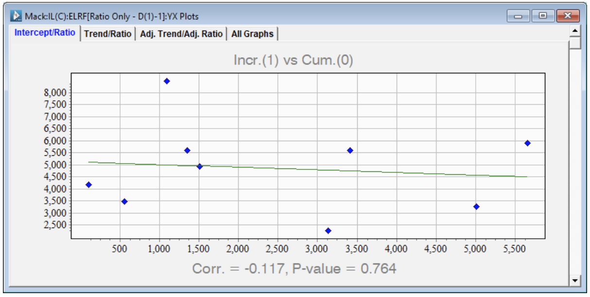
Here is a graph (right) of the incrementals in development year 1 versus the cumulatives in development year 0.
Note that the correlation is zero (slope not statistically significant). Equivalently b – 1 = 0.
In this case, the reduced model only contains an intercept term.
y(w) – x(w) = a + e(w) … (4)
In this model, the incrementals across the accident years are random numbers from a distribution with mean a, and variance, Var(e(w)). If e(w) has a constant variance, then the ordinary least squares estimate of a is the arithmetic average of the incrementals y(w) – x(w).
It turns out, if you graph the incrementals in any development period against the cumulatives in the previous period, you will note that there are no statistically significant correlations. All the b-1 parameters are statistically zero.
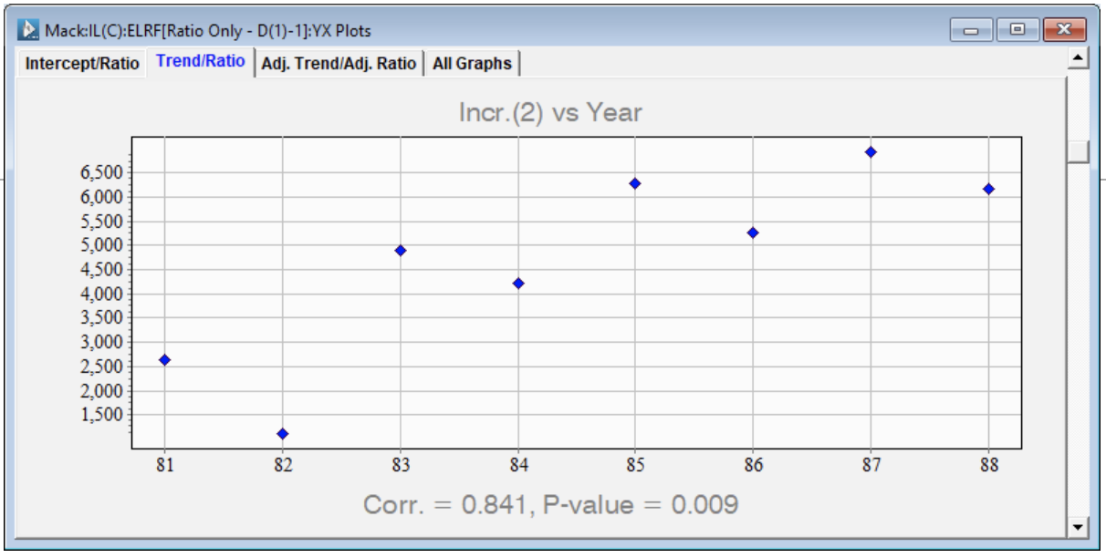
The assumption that the incrementals are random, might not be true. A case in point, is development period two. This suggests that we need to include an accident year trend parameter in model (3).
The equation that includes the intercept, accident year trend and slope can be written:
y(w) – x(w) = a0 + a1 * w + (b-1)*x(w) + e(w), … (5)
where a0 is the intercept, a1 is the accident year trend parameter and b-1 is the incremental coefficient.
The family of models included in the Extended Link Ratio Family (ELRF) are represented by equation (5) between each two consecutive development years. The significance of the parameters is determined by the data.
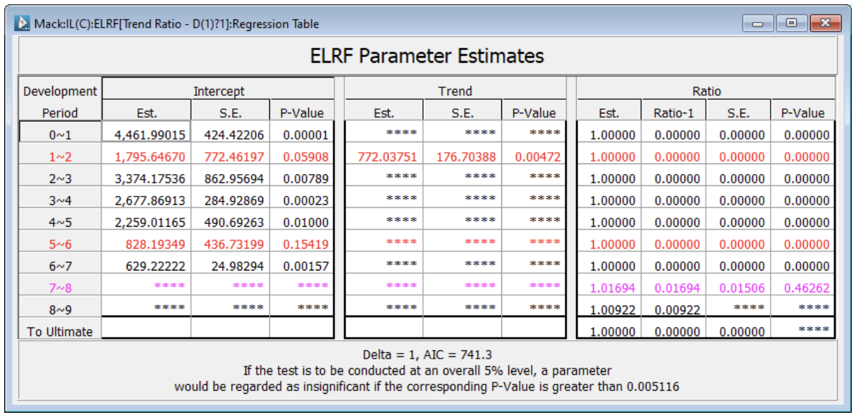
Link ratios have no predictive power for this incurred loss development array. The optimal combination of parameters uses simply an intercept term with the exception of the regression equation between development periods 1 and 2 where an accident year trend is also statistically significant.
Mack, T. (1993). Distribution-free calculation of the standard error of chain ladder reserve estimates. ASTIN Bulletin: The Journal of the IAA, 23(2), 213-225.
Murphy, D. M. (1994, March). Unbiased loss development factors. In CAS Forum (Vol. 1, p. 183).
Venter, G. G. (1998). Testing the assumptions of age-to-age factors. In Proceedings of the Casualty Actuarial Society (Vol. 85, pp. 807-847).
Volume weighted average link ratios do not distinguish between accident years and development years
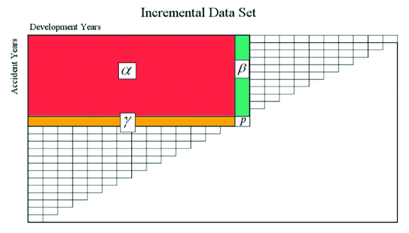
Consider any triangle with incremental values where:
- alpha denotes the sum of the values in the red rectangle,
- beta denotes the sum of the values in the green rectangle (one development year), and
- gamma is the sum of the values in the orange rectangle (one accident year).
Let p denote the incremental value projected for the accident year represented by the gamma values for the next development year.
The value alpha represents both the aggregate of the row sums in the red rectangle and the aggregate of the column sums.
The volume weighted average when you cumulate the triangle in the traditional way is (alpha + beta) / alpha. If you cumulate the triangle for each development year down the accident years, then the volume weighted average is (alpha + gamma) / alpha.
Accordingly:
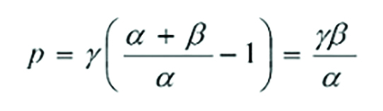
If you cumulate along the development years, and
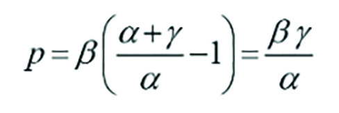
If you cumulate along the accident years. QED.
We know that development years are not like accident years.
CONCLUSION: Link ratios have got nothing to do with the structure of the data.
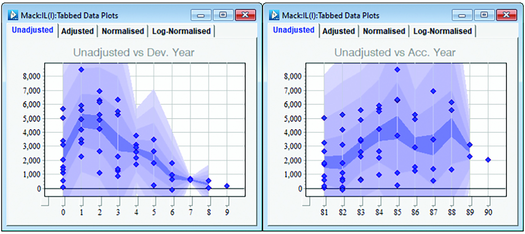
For the incurred array we plot the incremental values versus development year. We also plot the values versus accident year. Note the different structure.
Clearly, we expect any incremental loss development array to decay to zero, but you would not expect the same pattern down the accident years.