
Variability and Uncertainty
Variability and Uncertainty are different concepts and should not be used interchangeably.
Variability is a phenomenon in the physical world to be measured, analyzed and where appropriate explained.
- Sir David Cox
By contrast uncertainty is an aspect of knowledge.
(This quote is taken from: Section 2.4, Risk Analysis: A Quantitative Guide, by David Vose).
Uncertainty and variability are statistically very different, and it is common for them to be kept separate in risk analysis modelling.
A Best Estimate can only be assessed as best in the context of a probability distribution and the measurements of uncertainty and variability - supported by the data.
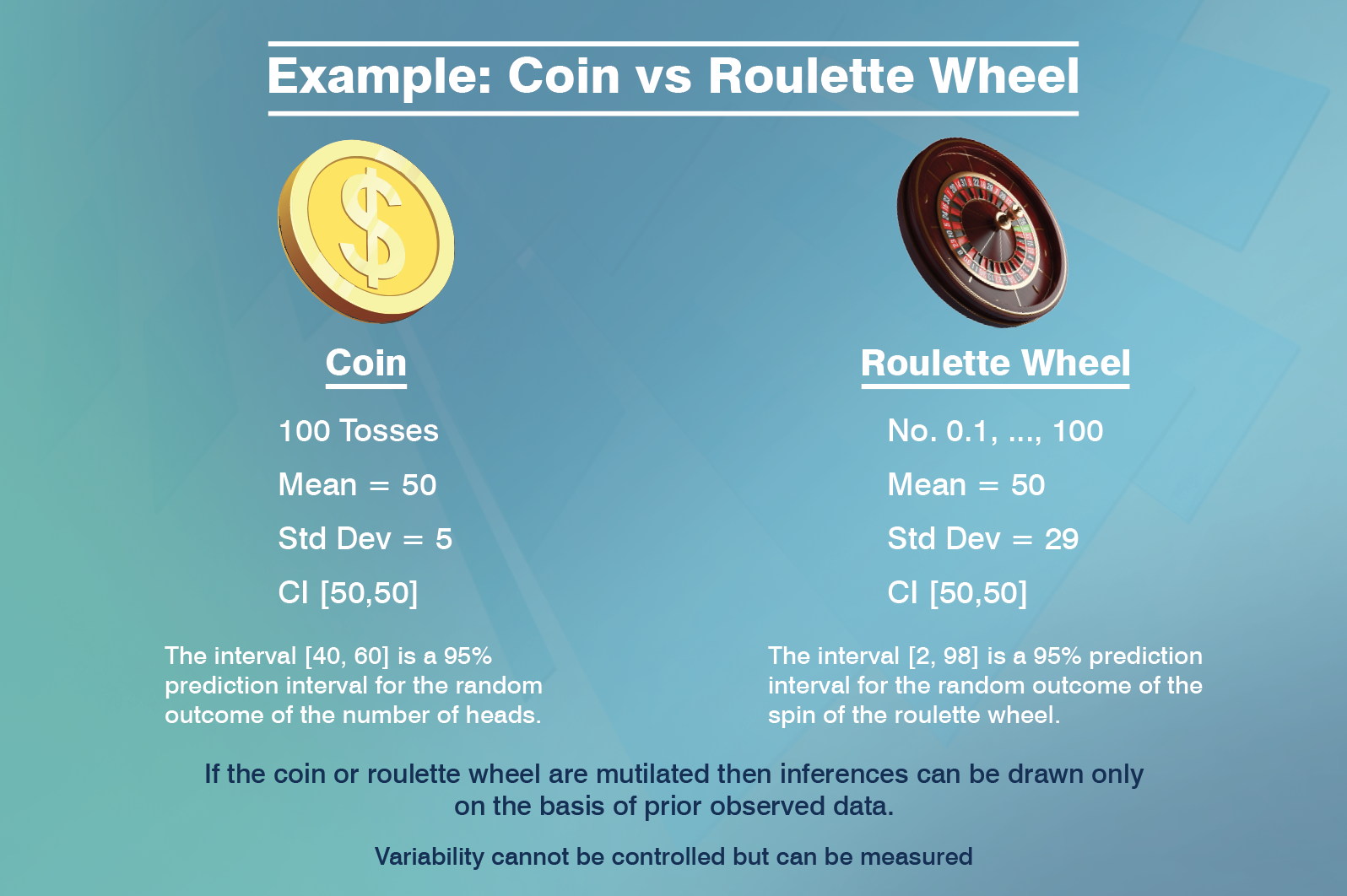
Let’s look at the example of a Coin vs a Roulette Wheel.
No Uncertainty about Variability
Example 1: Fair coin
When you toss a fair coin N times, you know the all the binomial probabilities exactly. There is no uncertainty in your knowledge about the variability of the coin.
If N equals 100 then:
The exact mean (of the number of heads) is 50.
The standard deviation is 5.
The 100% confidence interval of the mean is [50, 50] – we know it is a fair coin.
In (approximately) 95% of experiments with tossing the coin 100 times, the number of heads will be in the interval [40, 60]. The interval [40,60] is a prediction interval (of a random outcome).
(A confidence interval is an interval for a parameter. A prediction interval is an interval for a random outcome).
If you make the length of the prediction interval [40, 60] shorter, the probability reduces. In other words, we cannot reduce the variability in the coin – no matter how many experiments we do.
Example 2: Fair roulette wheel
Now, take a fair roulette wheel with 101 slots numbered from 0 to 100.
The probability of a particular outcome is 1/101.
The mean outcome of spinning the roulette wheel is 50, but the standard deviation is 29.
The 100% confidence interval for the mean is [50,50] – we know it is a fair roulette wheel.
The 95% prediction interval of a random outcome is [2, 98].
In both the examples above, our knowledge about the variability is perfect and the uncertainty about the variability is zero.
Would you charge the same premium for each risk – given that the mean is the same? Obviously not.
De Moivre’s gamblers ruin problem
If you charge the mean repeatedly (ie for every game) and do not have infinite capital, the probability of ultimate ruin is 1.
Accordingly, the mean alone does not reflect the true risk (just as illustrated in the examples above).
Uncertain knowledge about Variability
As soon as the coin or roulette wheel are mutilated, or even if we simply do not know whether it is indeed fair, inferences can only be drawn on the basis of past observed data.
In this case we have uncertainty about the variability.
Suppose in the coin example, before you toss the coin 100 times, you have data based on 10 prior tosses and you happen to observe 5 heads.
Now your estimate of the mean number of heads in 100 future tosses is still 50, but is subject to uncertainty.
Given that the true mean could be larger than 50, or smaller than 50, a 95% prediction interval will necessarily be wider than [40, 60].
Parameter uncertainty increases the width of a prediction interval.
A Best Estimate is meaningless without the associated measurement of variability.
Case study: Paid Loss development array
Let’s look at a case study of real life data.
The data are in the Workbook database supplied with ICRFS – Triangle Group: All 1M xs 1M. These data are medical malpractice data in the layer where paid losses are, in respect of individual losses, in the layer 1M to 2M.
If you open the triangle group and run the model called Good you obtain the following model display. It describes the trends in the three directions and the variances of the normal distribution versus development year. The model shows a high level of volatility by development period (see lower right hand side chart), along with high parameter uncertainty (see calendar year trends in particular).
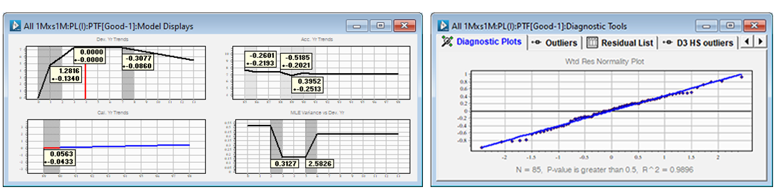
Given the residuals are normally distributed (above), we forecast normal distributions for each cell (and their correlations) going forward, then transform them to the corresponding log-normal distributions.
The mean and standard deviation of the log-normals are displayed in the forecast table with additional information.
Note that the forecasts are computed assuming that the true calendar year trend (going forward) is a realization from a normal distribution with mean 5.63% and standard deviation 4.33%.
The larger the variance of the normal distribution, the larger the mean of the corresponding log-normal.
We run the following four forecast scenarios sequentially (re-estimating the model between each step so extra lines are added in the log-book).
- Including parameter uncertainty and process variability (default forecast)
- Excluding parameter uncertainty
- Excluding process variability
- Excluding both parameter uncertainty and process variability
These parameters can be controlled in the forecast dialog in the marked locations:
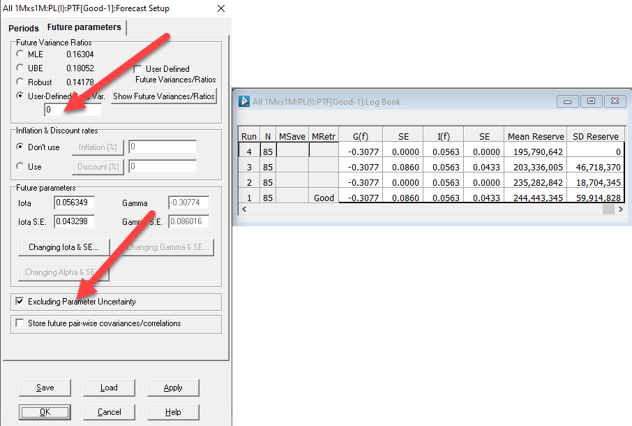
Note that the Total Reserve Mean and Total Reserve Standard Deviation of the first run – including parameter uncertainty and process volatility – are the largest.
The second run, excluding the parameter uncertainty, has a lower mean reserve to (1) and a significantly lower SD of the reserve distribution.
This is due to the high uncertainty about the future calendar year trend in particular.
In our example, the future calendar year trend (on a log scale) comes from a normal distribution with mean 5.63% and standard deviation 4.33%.
That is, the impact of inflation on the next calendar year is exp(iota) where iota comes from the N(0.0563, 0.0433^2).
The mean of exp(iota) = exp(0.0563 + ½ * 0.0433^2). The larger the uncertainty about the future parameter, the larger the mean.
This is the reason the mean payment increases when parameter uncertainty increases around the estimated mean parameters.
Excluding process variability (run 3), has a greater impact on the mean than run 2, but lower impact on the standard deviation of the reserve distribution.
As soon as all uncertainty and variability are removed from the calculation of the forecast, the standard deviation of the reserve distribution is 0 and the total reserve mean is the lowest projection of the four forecast scenarios.
The computation of the Best Estimate necessarily involves the measurement of uncertainty and variability. It is conducted in the context of probability distributions where any assumptions are supported by the data.