

In any loss development array, the calendar year (diagonal) trends project along the other two directions. That is, the accident years (rows) and development years (columns) are necessarily impacted by calendar year trends.
This is not a modelling choice. It is a structural property of the triangle.
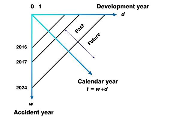
For convenience, we number development lags from zero.
Along the diagonal, any action – whether it is paid losses, case reserve estimates, or counts – is taken in the same year.
Social inflation in a given calendar year affects all prior accident years in respect of their resultant development year trends.
Algebraically, since:
t = w + d
We have:
(1+i)t = (1+i)w +(1+i)d
Where, i, denotes the inflation.
That is, a trend on t is a trend on w and a trend on d.
Deterministic Example
To illustrate, let’s look at a case where we generate paid losses using the following equation:
p(w,d) = exp(11.513 – 0.2d)
where d is the development year and w is the accident year.
On a logarithmic scale, this represents a straight-line with a slope of −20%, identical across all accident years.
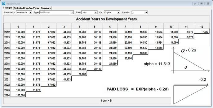
There are:
- no accident year trends and
- no calendar year trends.
It is easy to complete the square in this example.
Deterministic example with three calendar year trends
Let’s now add some known calendar year trends on a log scale.
- 10% from 2012 to 2016;
- 30% from 2016 to 2017; and
- 15% from 2017 onward
On a log scale trends are straight lines.
For accident year 2012:
- development years 0 through 4, the 10% projects along the development years so the resultant trend is -20% + 10% = -10%. As you move from one development year to the next, you’re also going to the next calendar year.
- development year 4 to 5, the 30% projects along the development years so the resultant trend is -20% + 30% = +10%.
- development years 5 onward the resultant trend is -5%.
For accident year 2013, the 30% trend kicks in one development year earlier (and so on).
Now we examine the impact of the calendar year trends for each development year across the accident years.
For each development year, stepping down accident years similarly you move to the next calendar years.
For example, if you take development year 2, it’s 10% for two years, then 30% for one year, and 15% thereafter.
The model relates every cell in the triangle to every other cell. This reflects the structural dependence implied by the triangle itself. Any coherent reserving model should describe the mathematical features that underpin the generating process.
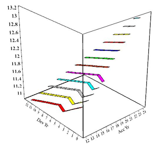
The resultant trends for all the accident years are depicted below. The bottom red line is the accident year 2012; the top maroon line is accident year 2023.
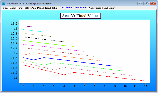
Notice that in the graph that the 30% trend always kicks in one development year earlier.
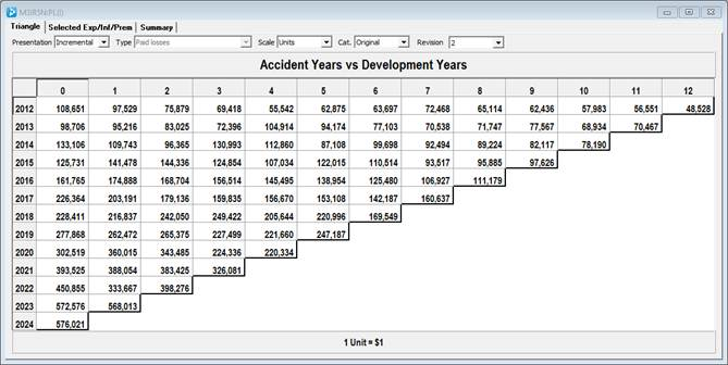
Imposing the above calendar year trends onto the original data above leads to:
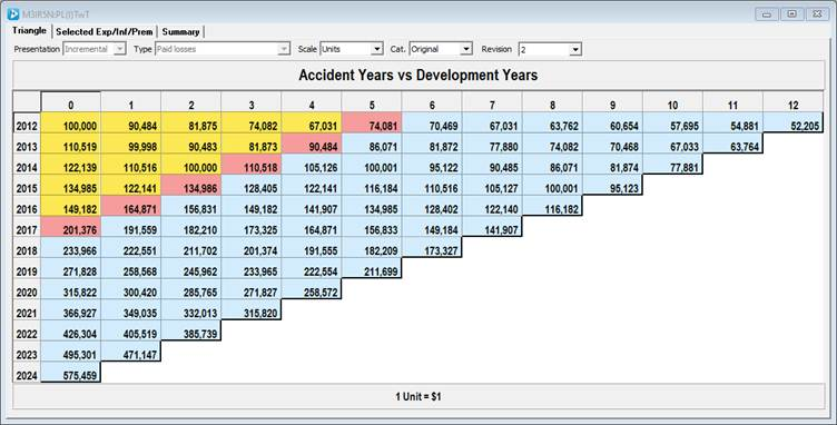
By eye it is now harder to complete the square. The shaded areas show the regions corresponding to the 10% (yellow), 30% (red) and 15% (blue) respectively.
The structure of the data can be represented by three graphs.
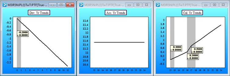
The resultant trends in three dimensions look like:
Adding variability around the trend structure
Let’s take the data above with the calendar year trends and add some randomness to the trend structure.
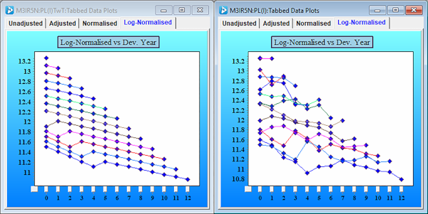
The chart on the right shows that the randomness has masked the trend structure depicted on the left chart.
Even with a small amount of randomness applied to the losses on a log scale in each cell, by visual inspection alone it becomes extremely difficult to recover the underlying trend shifts.
You need a statistical modelling framework for separating trends in the data from variability around the trend structure.
NB: real data typically exhibit much more variability around the trends than this illustrative example.
Model Decomposition
If we measure the trends and variability about the trends in the data we obtain the model display.
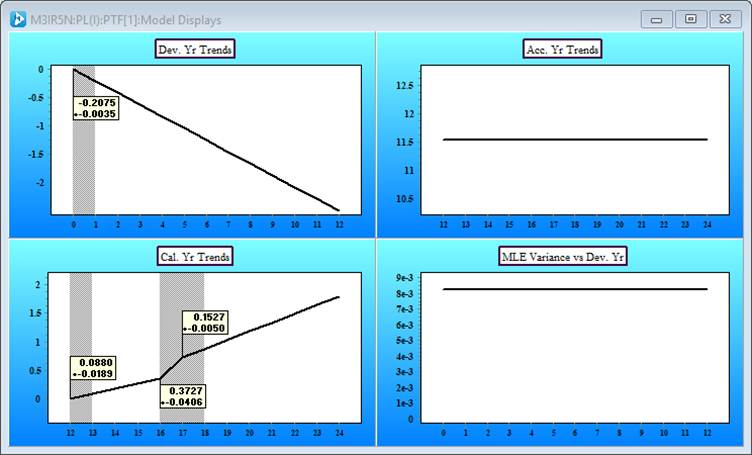
The four model charts are as follows:
- Top left – development year trends;
- Top right –accident year trends (here constant)
- Bottom left – calendar year trends (three changes estimated)
- Bottom right – the variability around the trends
Now we have estimates of the trend changes, with their uncertainty, along with an estimate of the variability about the trend (bottom right). We quantify the variability in terms of distributions. The modelling framework separates the structural trends from variability.
The distribution of variability around the trend structure on a log scale is an integral part of the model.
This decomposition allows:
- Identification of past structural trend changes
- Quantification of uncertainty of parameters
- Distribution of variability around the trend structure
- Construction of forward-looking scenarios
For example, modelling the data as at end-2017 would have clearly revealed the large 2016–2017 calendar year shock. If this was attributed to law reform to be conservative you may continue with that trend for one more year before reverting to the old trend.
In subsequent articles, we will discuss the Variation in Mean Ultimate metric which can be used in reserve releases if the assumptions going forward turn out to be too conservative.
Closing Observations
Without proper decomposition into parsimonious trends and variability around those trends - risks cannot be assessed.
Models including calendar trends do not add unnecessary sophistication, rather they are an essential feature as they reflect real-world structure.
To learn more about Insureware’s Probabilistic Trend Family modelling framework see the PTF brochure.
Side note about inflation
Inflation, whether economic or social, operates multiplicatively on the dollar scale.
On a logarithmic scale it is additive.
Accordingly, on a log scale, inflation only changes the mean, not the variance.
For Poisson and Over-Dispersed Poisson models on a log scale the variance is a function of the mean.
This is not aligned with the property of inflation and accordingly rules both the Poisson and Over-Dispersed Poisson distributions out.
More on this in a subsequent post.