

Would you have lost money?
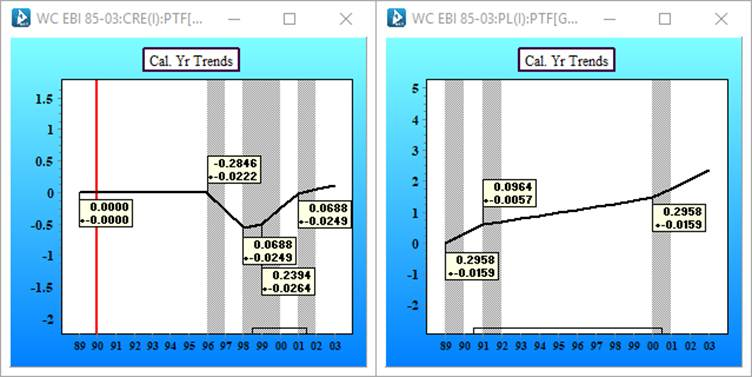
The left display shows calendar year trends in the Case Reserve Estimates, whereas the right display shows calendar year trends in the Paid Losses.
In the years 1996 to 1998 the company was reducing Case Reserve Estimates by 28.46%+_ a year, yet the Paid Losses were always increasing.
From 1998 onwards, the Case Reserve Estimates started increasing.
Can you pick the year the company was sold?
The purchaser required a stop loss on reserves as part of the transaction.
The reinsurers providing that cover ultimately lost a significant amount of money as they materially underestimated the risk.
Why?
Below is a display of the calendar year trends in the incremental Incurred Losses.
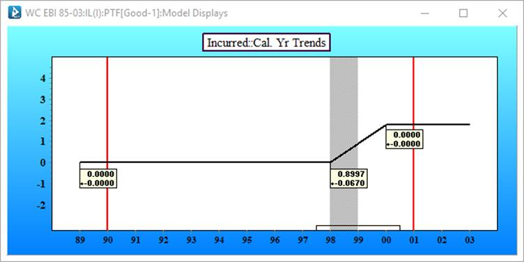
Suddenly, from 1998 through 2000, an 89.97% trend appears in the Incurred Losses – despite no sign of any issues prior to 1998! Most likely the increase is due to Case Reserve Estimates increasing.
Let’s look at Paid Losses and Case Reserve Estimates at year end 1998
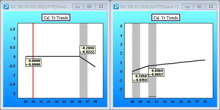
In the Case Reserve Estimates a negative trend is measured from 1996 – 1998; whereas there was no change in trend in the Paid Losses. Coincidentally, the portfolio was put on the market in 1996.
During the period the seller was negotiating the sale, the Case Reserve Estimates decreased.
Consider the calendar year trends in the incremental Incurred Losses as at year end 1998.
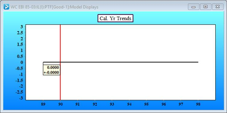
The calendar year trend is zero for the whole period – neither increasing or decreasing. Everything looks good; nothing to see here – certainly no points of potential concern.
Based on the information from the incremental Incurred Losses, there would be little reason to suspect the reserves.
The story as to why the Case Reserve Estimates are reducing becomes critical – and that story vanishes if only the Incurred Losses are modelled.
The portfolio was sold in 1998.
Simpson’s Paradox
This phenomenon is closely related to Simpson’s paradox. Namely, that trends present in individual data series disappear or reverse when the data are aggregated.
Incurred = Paid + Case Reserve Estimates
Therefore, if trends in the individual series move in different directions (like in this example), modelling Incurred Losses alone can give a misleading impression of stability. Underlying issues, present in the data, may be masked until corrective action is too late.
Summary
If you only analyse Incurred Losses, then important information critical for strategic decision making or risk assessment will disappear.
Case Reserve Estimates are inherently soft data – varying with company policy, management strategy, and current views on financial conditions.
Paid Losses are what the company actually paid. Barring accounting errors, this is hard data – it is also required to project future cash flows for IFRS 17 purposes.
When Paid Losses and Case Reserve Estimates are modelled separately, the underlying drivers of trends are revealed – providing valuable information and potential warning signals. It is the relationship between these two processes that carries risk insight.