In the presentation, "Integrating Reserve Risk Models into Economic Capital Models" by François Morin of Towers Perrin, the Solvency II one-year risk horizon is measured as the sample variance of the difference between estimates of ultimates today and one year from now. François Morin of Towers Perrin provides several methods of calculating the variance of the change in estimate.
"Under Solvency II the one-year risk horizon is defined as the change in the estimate, one year hence, generally measured as the sample variance of the difference between the deterministic ultimate's one year from now and the deterministic ultimate's today." (see page 20 "Integrating Reserve Risk Models into Economic Capital Models").
We discuss the consistent and sound statistical methodology for calculating the variation in estimates of ultimates conditional on the next calendar years' data. The relationship between these estimates, consistent estimates of prior year ultimates on updating (next valuation period), and loss reserve increases on updating is discussed in detail here. Note that our approach also applies to the aggregate of multiple LOBs.
Calculating variation in ultimates conditional on next calendar years' data (Conditional Statistics)
Let Ult. denote the Ultimate and CY represent the next calendar year's paid losses.
| Step 1: | Using the model obtain the expectation of the ultimate E[Ult.] and variance of ultimate Var[Ult.], |
| Step 2: | Using the model simulate the next CY's losses. |
| Step 3: | Re-estimate the model using the array with the additional CY's data and compute accident year ultimates. |
| Step 4: | Repeat Step 2 and Step 3 N times. |
For each simulation Step 3 computes E[Ult.|CY] and Var[Ult.|CY] using the model on the updated array.
The N simulations give us estimates of E[E[Ult.|CY]], E[Var[Ult.|CY]] and Var[E[Ult.|CY]].
Provided forecast assumptions (based on the model) are consistent on updating (see previous sections), we also have
| Var[Ult.] | = | E[Var[Ult.|CY]] + Var[E[Ult.|CY]], and |
| E[E[Ult.|CY]] | = | E[Ult.], |
François Morin of Towers Perrin mentions "the change in the estimate one year hence" which is equivalent to:
| Var[E[Ult.|CY]] | = | Var[Ult.]- E[Var[Ult.|CY]]. |
In respect of the identified models in the PTF and MPTF modelling frameworks there is no need to conduct simulations as the above mentioned formulae can be computed analytically using the identified parametric models. The statistics include both process variability and parameter uncertainty.
We include two Forecast Summary tables from ICRFS™, one from the aggregate of multiple long tail LOBs and the other Private Passenger Automobile (PPA).
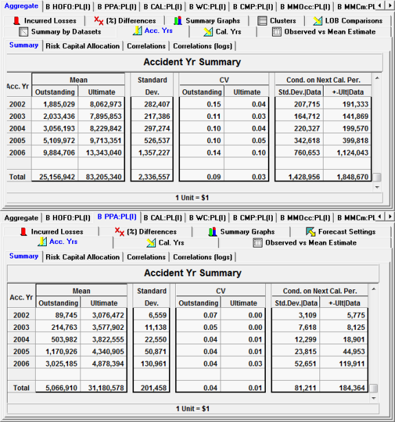
+-Ult|Data refers to SD[E[Ult.|CY]] and Std.Dev|Data to Sqrt(E[Var[Ult.|CY]]).
Consistency depends on whether the predicted forecast assumptions for the next year and following a) occur for the next year and b) that the same forecasting assumptions used previously for the following years are applied in the subsequent forecast. Any change in assumptions will make prior year ultimates on updating inconsistent. See here for more details.
Variation in Ultimates and the associated conditional statistics do not provide sufficient descriptors of the risk margin or cost of capital as required by Solvency II. Furthermore, calculating conditional statistics and variation in ultimates by using the Mack and related methods (including Bootstrapping) are inherently flawed. For a more detailed discussion of the paper by François Morin of Towers Perrin please click here.
See here for a demonstration video illustrating Solvency II metrics and consistency on updating.