The Mack Method and associated Bootstrap Predictions

Introduction

The Mack method in conjunction with the bootstrap is used by many practitioners to obtain loss reserve prediction distributions.

This approach is often very misguided and can give grossly inaccurate reserve indications.

According to Francois Morin ("Integrating Reserve Risk Models into Economic Capital Models"):

"Bootstrapping utilizes the sampling-with-replacement technique on the residuals of the historical data",

and

"Each simulated sampling scenario produces a new realization of "triangular data" that has the same statistical characteristics as the actual data." (Emphasis added)

This is worth repeating.

"...that has the same statistical characteristics as the actual data."

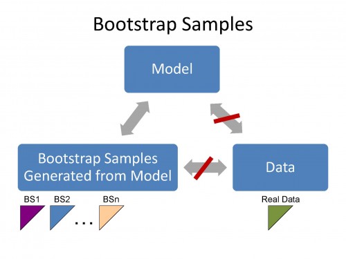
Bootstrap samples have the same statistical characteristics as the actual data

only

if the model has the same statistical characteristics as the actual (real) data.

The bootstrap samples have the same statistical features as the Model. If the Model does not have the same statistical features as the data then the bootstrap samples cannot have the same statistical features as the data. Accordingly, we can use the bootstrap technique to test the validity of the Model (for the data).

See real life examples in demonstration video chapter 10.

The Mack method, the Murphy method and related methods produce Bootstrap (pseudo) samples that have statistical features (characteristics) that are not related to the actual data. This is because these methods cannot capture nor describe the volatility in real data.

The Mack method is a regression formulation of volume-weighted average (Chain Ladder) link ratios and is the default (starting) model in the Extended Link Ratio Family (ELRF) modelling framework of ICRFS-Plus.

The ELRF modelling framework, that includes the Mack method amongst its numerous methods, is described here. More technical details are given, using a real life example in the demonstration video 1.2.

The Mack method often has standardized residuals with much structure, that is, they are not random. It is not only that the bootstrap technique does not apply in such a situation, but the model fails to describe the volatility in the data and accordingly does not have much predictive power. [See video demonstrations 1.2 and 2.1-2.5].

The bootstrap is a way to obtain an approximate sampling distribution for a statistic (a function of the data).

In the context of modelling loss development arrays, if the data satisfy parametric assumptions and a suitable parsimonious model fits a distribution to each cell (as in the Probabilistic Trend Family (PTF) modelling framework), the bootstrap technique will yield approximately the same predictive distributions as the parametric model.

A general and detailed discussion of the bootstrap is given in the paper by Barnett and Zehnwirth (2007). This paper discusses methodological issues which are often overlooked even in applying the bootstrap to otherwise careful refinements of the Mack method. In particular the need to look at a model's prediction residuals before giving any credence to the bootstrap distribution associated with its forecast.

It is predictive distributions and prediction intervals that are generally of prime interest to insurers (because they pay the outcome of the process, not its mean).

The bootstrap is not a model identification procedure. It does not in any way improve the model- it does not make a bad model good.

Accordingly, it does not avoid the need for assumptions, nor for checking those assumptions. It suffers from essentially the same problems as any other means of finding predictive distributions and sampling distributions. For example, because reserving requires prediction into not-yet-observed calendar periods, model inadequacy in the calendar year direction becomes a serious problem.

In particular, the most popular actuarial techniques based on link ratios and their derivatives- those most often used with the bootstrap - don't have any parameters in that direction, and are frequently mis-specified with respect to the behavior of the data against calendar time.

Further, some commonly used versions of the bootstrap can be sensitive to over parameterization - and over parameterization is a common problem with standard actuarial models.

It is critical to carefully assess both the assumptions and the predictive performance of the model, or the bootstrap prediction intervals can be meaningless.

The Bootstrap

The bootstrap was devised by Efron (1979), growing out of earlier work on the jackknife. He further developed it in a book (Efron, 1982), and various other papers. There are numerous books relating to the bootstrap, such as Efron and Tibshirani (1994). A good introduction to the basic bootstrap may be found in Moore et al. (2003), which can be obtained online.

In the original form of the bootstrap the data itself is re-sampled, in order to get an approximation to the sampling distribution of some statistic of interest, in order to make inference about a corresponding population statistic.

More complicated models can be bootstrapped by re-sampling residuals. This is the kind of bootstrapping used in most reserving applications.

A simple residual re-sampling bootstrap

Consider a set of observations y=( y1, ..., yn)

Suppose we want to find the distribution of a statistic S(y), a function of the data y.

Here is a simple bootstrap algorithm:

Repeat 3. 4. and 5 to generate many bootstrap values S(y*). The bootstrap values for S form an empirical distribution.

Note that a key assumption here is that the standardized residuals ei are random and do not exhibit structure.

We can use these bootstrap samples based on re-sampled residuals to obtain sampling properties of various statistics - such as standard errors of parameter estimates.

The bootstrap can also be adapted to give prediction intervals and distributions.

Further modifications are required to use this to produce prediction intervals.

Example 1: LR high data

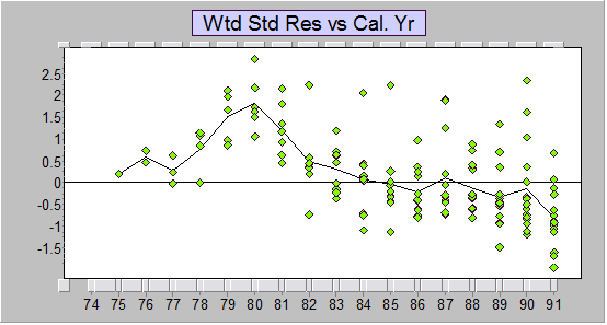
Here not only are the bootstrap predictions useless but the reserve indications given by the Mack method are at least 80% too high!

The standardized residuals versus calendar years of the Mack method (Chain ladder, equivalently, volume weighted average link ratios) to the data are given below. As you can see, there's a lot of structure and accordingly randomly reallocating (i.e. bootstrapping) the standardized residuals is meaningless.

Residuals represent the trend in the data minus the trend in the method. The Mack method does not have any descriptors of the trends captured in the data but we can tell immediately that the trend in the method (for these data) is much higher than the trend in the data (data trend minus method trend is negative), and accordingly the predictions are much too high.

See video demonstration 2.5 LR High that discusses much improved ELRF type models and optimally identified PTF models for the paid losses, case reserve estimates and the number of claims closed, and their inter-relationships. The video explains why the Mack predictions are at least 80% too high.

Example 2: ABC data

The data are Worker's Compensation data for a large company studied in Barnett and Zehnwirth (2000).

For more technical details in respect of bootstrapping the residuals for this example, see the paper Barnett and Zehnwirth (2007).

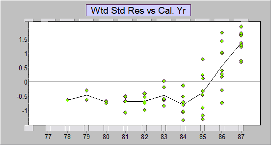
Below are the standardized residuals versus calendar year. Observe that there is much structure in the residuals (calendar year trend change around 1985) and the method under-fits the last two calendar years (and over-fits the earlier years).

[Some actuaries might only apply Mack to the last three calendar years. However, the method still does not capture the trend (since the cumulatives in the final three years include incrementals from the old trend) and even if it did you would have no description of what it is].

One major difficulty with the common use of the Mack (chain ladder), and indeed any link ratio type method and derivative thereof, is that there is no opportunity to apply proper judgment of the future calendar year trends. The practitioner lacks information about past calendar year trends that would inform scenarios relating to the future calendar year trend behaviour. And this is only one of a number of critical issues.

The demonstration video 2.2 ABC considers an alternative optimally identified PTF model that replicates the true volatility in the data. Simulated triangles from the fitted probabilistic model cannot be distinguished in respect of volatility from the real triangle. In the context of PTF type models the actuary has control on future assumptions that can be related to current and past volatility in the business.

References

Barnett and Zehnwirth (2000) Best Estimates for Reserves, PCAS LXXXVII, 245-303.

Barnett and Zehnwirth (2007) The need for diagnostic assessment of bootstrap predictive models, Insureware technical report.

Efron, B. (1979) Bootstrap methods: another look at the jackknife, Ann. Statist., 7, 1-26.

Efron, B. (1982) The Jacknife, the Bootstrap and Other Resampling Plans. vol 38, SIAM, Philadelphia.

Efron, B. and Tibshirani, R. (1994) An Introduction to the Bootstrap, Chapman and Hall, New York.

England and Verrall (1999) Analytic and bootstrap estimates of prediction errors in claims reserving, Insurance: Mathematics and Economics, 25, 281-293.

Moore, D. S., G.P. McCabe, W.M. Duckworth, and S.L. Sclove (2003), "Bootstrap Methods and Permutation Tests," companion chapter 18 to The Practice of Business Statistics, W. H. Freeman (also 2003).http://bcs.whfreeman.com/pbs/cat_140/chap18.pdf

Pinheiro, P.J.R., Andrade e Silva , J. M. and Centeno, M. L. (2003) Bootstrap Methodology in Claim Reserving, Journal of Risk and Insurance, 70 (4), pp. 701-714

Zehnwirth, B (1981) The jackknife and the variance part of the credibility premium. Scand. Actuarial J., Vol. 4, 245-50.