by Glen Barnett and Ben Zehnwirth
This article presents regression methodology that can be used to test assumptions made by the standard ratio techniques. The methodology is easy to follow and could be implemented simply in a spreadsheet program.
This note describes regression methodology for calculating development factors optimally and testing their appropriateness. The methodology can also be used to discriminate between two approaches to forecasting: application of selected factors to cumulative data and trending the incremental data down each development period. In each case the data may also be adjusted by accident period exposures.
The methodology demonstrates the lack of predictive power of development factor techniques for most, if not all, cumulative arrays.
The most widely used approach for loss (claims) reserving is based on the computation and subsequent selection of development factors associated with an array of cumulative values. Selection of development factors is often based on some ad hoc averaging method (e.g. the chain ladder technique), without any specific optimally criterion being adopted.
It turns out that many of the common averaging methods give development factors that can also be obtained as regression estimates. This means that well-known regression methodology can be applied to determine optimal development factors and standard errors of forecasts. More importantly, the regression methodology provides the framework for testing whether the data supports the assumptions contained in the model.
Mack (1994) shows that the standard chain ladder approach can be formulated as
| E[y(i)|x(i)] | = | bx(i), |
| Var[y(i)|x(i)] | = | sigma2x(i) |
where,
y(i) is the cumulative at accident year i, development j,
x(i) is the cumulative at accident year i, development j-1,
b is the development factor (between development period j-1 and j).
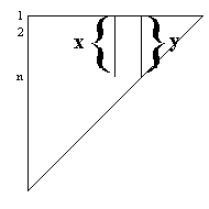
Murphy (1994) writes this model as an equivalent weighted regression model,
y(i) = bx(i) + e(i), Var(e(i)) = sigma2x(i) - (1)
The weighted least squares estimates of the b parameters between every two contiguous development periods are the chain-ladder ratios. That is,
| b (hat) | = | Sum{x(i)y(i)/x(i)} / Sum{x(i)} |
| = | Sum{y(i)} / Sum{x(i)} - (2) |
The model assumes that the expectation of y(i), given x(i) is bx(i). That is, if x(i) is large, the mean of y(i) will be large, and if x(i) is small, the mean of y(i) will be small. This assumption can be diagnostically tested by examining a graph of the weighted standardised residuals of all the pairwise regressions versus the corresponding fitted values. A downward slope, as depicted in the example below, is diagnostic evidence that this assumption is not satisfied.
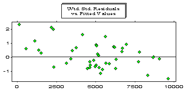
Note that the large values are overfitted whereas the small values are underfitted. This example is based on the Reinsurance Association of America Facultative Business incurred losses array for General Liability. This array is also analysed by Mack (1994).
The graph below depicts (for the Mack (1994) data) the cumulative in development period 1 versus the cumulative at development period 0. Note that a (positive) intercept is required.
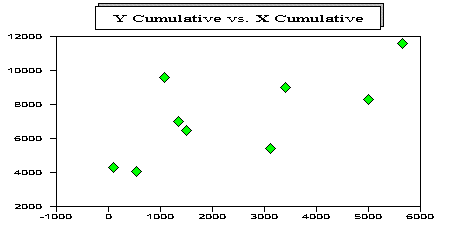
Murphy (1994) suggested the addition of an intercept parameter in order to alleviate this deficiency,
y(i) = a0 + bx(i) + e(i), - (3)
He also included a weighting parameter, delta, so that the variance of the error is sigma2x(i)delta, and considered the cases delta = 0, 1 and 2. An optimal value of delta can be chosen by using a discriminatory statistic such as AIC.
Venter (1996) suggested that equation (3) be rewritten as
y(i) - x(i) = a0 + (b-1)x(i) + e(i), - (4)
If the estimate of the intercept a0 is significant, but the estimate of the development factor b is not significantly different from one, it follows that the cumulative x(i) has no predictive power for the incremental, y(i)-x(i), and hence is a poor predictor for the cumulative, y(i). In this case a graph of the incremental y(i)-x(i), versus the previous cumulative x(i) will exhibit randomness.
The graph below depicts (for the Mack (1994) data) the incremental data in development period one versus the cumulative in development period 0. Note the zero correlation.
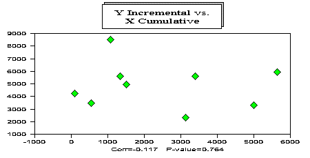
The model then reduces to
y(i) - x(i) = a0 + e(i), - (5)
That is, the model fits the average incrementals, and so the forecasts of the incrementals for the specific development period will just be a weighted average of the incrementals in that development period. This approach has more predictive power (if b=1) than multiplying cumulatives by development factors (less one).
Venter (1996) shows that the development factors for the Reinsurance Association of America Facultative Business incurred losses array for General Liability are not significantly different from 1 (provided there is an intercept term in the model).
If the incrementals for a particular development period are increasing down the accident years, then in model (4) the parameter (b-1) will be significantly different from zero. However, if we introduce a trend parameter for the incrementals,
y(i) - x(i) = a0 + a1i + (b - 1)x(i) + e(i), - (6)
we will usually find that the development factor (b) is again not significantly different from one. That is, after adjusting the incrementals by the estimate of the trend parameter (a1), the previous development period cumulatives x(i) have no predictive power for the next devlopment period incrementals.
We have so far considered two cases: incrementals for a particular development period have a zero trend, and incrementals have a constant trend. The case encountered most often in practice involves a trend change along the payment periods (diagonals). This means that as you look down each development period, the change in trend will occur in different accident years. Consequently, none of the above models can capture these trends. The weighted standardised residuals depicted below come from applying model (6) independently to each pair of development years for a certain real-life cumulative paid loss array for a Worker’s Compensation portfolio. Note the trend before 1984 is different from (lower than) than the trend after 1984.
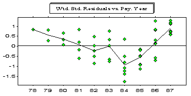
The types of models described by equation (6) can be used to diagnostically identify payment period trend changes, but cannot estimate these trend changes or forecast with them. These models form a bridge to models that also include payment period trend parameters.
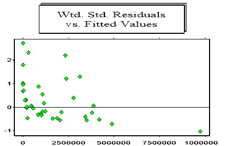
It is important to note that these models also make the implicit assumption that the weighted standardised errors, e(i)/sigmax(i)delta/2 come from a normal distribution. If the assumption is true, the estimates of the regression parameters are optimal. If the assumption is not true, the estimates may be very poor. This normality assumption is rarely true for loss reserving data ? in fact, the weighted standardised residuals are generally skewed to the right, suggesting that the analysis should be conducted on the logarithmic scale. The graph below illustrates the skewness of a set of weighted standardised residuals based on chain ladder ratios. The positive weighted standardised residuals are further from zero than the negative ones. If the normality assumption were correct, the plot would look roughly symmetric about the zero line.
In summary, using the above regression methodology, you will discover that for most real loss development arrays of any data type, standard development factor techniques are inappropriate. Analysing the incrementals on the logarithmic scale with the inclusion of payment period trend parameters has more predictive power.
Finally, but importantly, the estimate of a mean forecast of outstanding and corresponding standard deviation based on a model are meaningless unless the assumptions contained in the model are supported by the data.
References
Mack T. (1994). Which stochastic model is underlying the chain ladder method? Insurance: Mathematics and Economics, Vol 15 No. 2/3. 133-138.
Murphy D. (1994). Unbiased Loss Development Factors. Proceedings of the Casualty Actuarial Society, Vol LXXXI No. 144-155, 154-222.
Venter G. (1996). Testing assumptions of age-to-age Factors. Draft Report, Instrat/Sedgwick Re, New York.
