Fundamentals of correlations, linearity, and regressions
The idea of correlation arises naturally for two random variables that have a joint distribution that is bivariate normal. For each individual variable, two parameters a mean and standard deviation are sufficient to fully describe its probability distribution. For the joint distribution, a single additional parameter is required the correlation.
If X and Y have a bivariate normal distribution, the relationship between them is linear; the mean of Y, given X, is a linear function of X. That is,
E(Y|X) = a + bX + e
The variance of the "error" term e does not depend on X.
However, not all variables are linearly related. Suppose we have two random variables related by the equation
S = T2
where T is normally distributed with mean zero and variance 1.
What is the linear correlation between S and T?
Linear correlation is a measure of how close two random variables are to being linearly related.
In fact, if we know that the linear correlation is +1 or -1, then there must be a deterministic linear relationship
Y = a + bX between Y and X (and vice versa).
Note that a linear relationship does not indicate a causal relationship between X and Y.
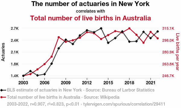
Developing a story around two apparently connected series (the linear correlaion is 0.9 above) is a dangerous, if amusing, passtime.
If Y and X are linearly related, and f and g are functions, the relationship between f(Y) and g(X) is not necessarily linear, so we should not expect the linear correlation between f(Y) and g(X) to be the same as between Y and X.
Correlation and Regression
Correlations measured before and after regression can be very different. Hence if we want to assess the effective correlation between two series we must first remove trends (the predictable portion) and measure the correlation of the residuals (the random components.)
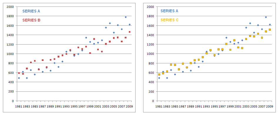
Consider the series A, B and C. Each has a linear trend, B and C appear quite similar. The correlation between A and B is 0.91 and between A and C is 0.97. Are A and B related? Are A and C related?
De-trending the series
Removing trends from the series, in this case by linear least-squares regression separates the predictable part from the random component.
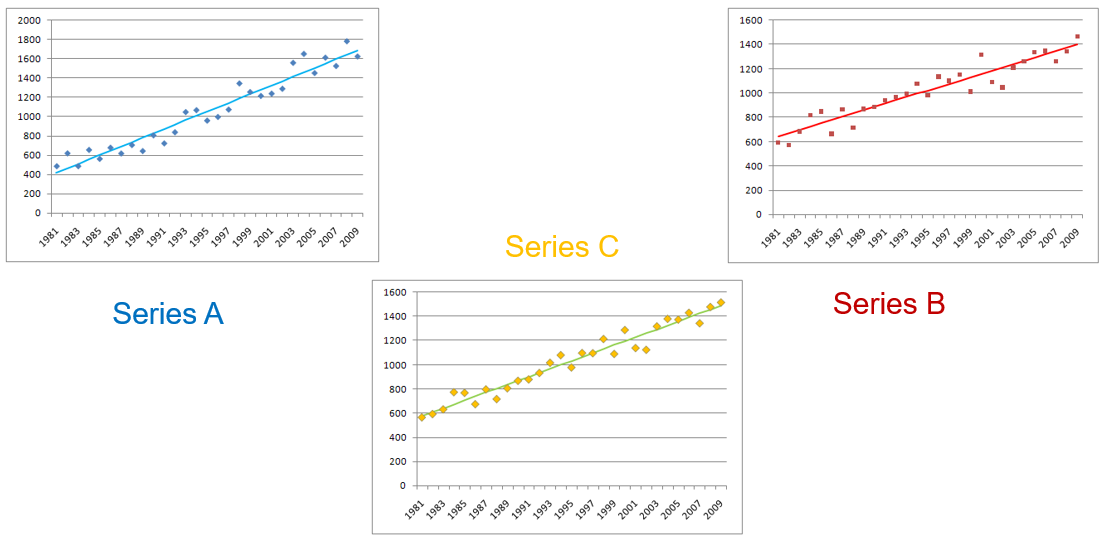
Compute the correlation of the residuals = the random component of each series.

Conclusion:
The series A and B merely share a common positive trend. There is no apparent causal or predictive relation between them. Series A and C exhibit a positive correlation. Information about the next value of C does have a significant bearing on prediction of the next value of A.
Scaling up to a full model for complex data
Models for more complex data, such as loss arrays, will include such elements as multi-directional and multi-parameter trends and heteroscedasticity. Furthermore, where significant correlations are detected modelling needs to take account of the effect of these for parameter estimates.
Ideally, model frameworks should have the following features:
(a) Models reflect the important structural characteristics of the data.
(b) Model parameters are readily interpretable.
(c) Feedback mechanisms (bi-directional causality) are included.
(d) Stationarity does not have to be assumed.
(e) On-line model maintenance and updating on receipt of additional information.
See more at how to calculate correlations between multiple Lines of Business on the process of detrending and calculating volatility correlations.
Ref: Sherris M.; Tedesco L.M.; Zehnwirth B. Investment Returns And Inflation Models: Some Australian Evidence, British Actuarial Journal Vol. 5, No. 1, 1999.